Understanding precision, accuracy, and tolerance of geospatial datasets: an example based on the usage of GNSS receivers
Appendix 1: how to manage errors in observations
This text is mainly extraxted from Ghilani, C. D. and P. R. Wolf. 2014. Elementary Surveying: An Introduction to Geomatics. Prentice, Hall Publishers, Upper Saddle River, NJ. Chapter 3, Theory of Errors in Observations
Surveyors (geomatics engineers) should thoroughly understand the different kinds of errors, their sources and expected magnitudes under varying conditions, and their manner of propagation. Only then can they select
instruments and procedures necessary to reduce error sizes to within tolerable limits. Of equal importance, surveyors must be capable of assessing the magnitudes of errors in their observations so that either their acceptability can be verified or, if necessary, new ones made.
By definition, an error is the difference between an observed value for a quantity and its true value, or:
\[E = X – \overline{X}\]
where E is the error in an observation, X the observed value, and X̄ its true value.
Errors in observations are of two types: systematic and random.
Systematic errors, also known as biases, result from factors that comprise the “measuring system” and include the environment, instrument, and observer. So long as system conditions remain constant, the systematic errors will likewise remain constant. If conditions change, the magnitudes of systematic errors also change. Because systematic errors tend to accumulate, they are sometimes called cumulative errors. Conditions producing systematic errors conform to physical laws that can be modeled mathematically. Thus, if the conditions are known to exist and can be
observed, a correction can be computed and applied to observed values.
Random errors are those that remain in measured values after mistakes and systematic errors have been eliminated. They are caused by factors beyond the control of the observer, obey the laws of probability, and are sometimes called accidental errors. They are present in all surveying observations. Random errors are also known as compensating errors, since they tend to partially cancel themselves in a series of observations.
Probability may be defined as the ratio of the number of times a result should occur to its total number of possibilities.
In physical observations, the true value of any quantity is never known. However, its most probable value can be calculated if redundant observations have been made. Redundant observations are measurements in excess of the minimum needed to determine a quantity. For a single unknown, the most probable value in this case is simply the arithmetic mean, or:
\[\overline{M}= \frac{\sum M}{n}\]
where M is an individual mesurement and n the total number of observations.
A residual is the difference between the most probable value and any observed value of a quantity:
\[\nu=\overline{M}-M\]
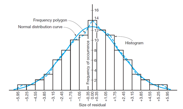
To analysethe distribution of the residuals, is useful to plot them on an histogram showing the sizes of the observations (or their residuals) versus their frequency of occurrence. The frequency polygon (or the curve that represent it, the blue dashed in the below figure), in case of normally distributed group of errors, has a “bell shape” and it is normally referred as a normal distribution curve. In surveying, normal or very nearly normal error distributions are expected.
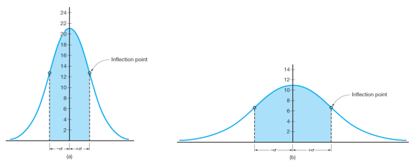
If the same type of observations is taken using better equipment, smaller errors would be expected and the normal distribution curve would be similar to that in Figure 8(a). Compared to Figure 8(b), this curve is taller and narrower, showing that a greater percentage of values have smaller errors, and fewer observations contain big ones. Thus, the observations of Figure 9(a) are more precise.
Statistical terms commonly used to express precisions of groups of observations are standard deviation and variance. Standard deviation is defined as following:
\[\sigma=\pm\sqrt{\frac{\sum\nu^{2}}{n-1}}\]
where σ is the standard deviation of a group of observations of the same quantity, ν the residual of an individual observation, and n the number of observations.
Variance is equal to the square of the standard deviation.
Figure 9 is a graph showing the percentage of the total area under a normal distribution curve that exists between ranges of residuals (errors) having equal positive and negative values. The abscissa scale is shown in multiples of the
standard deviation. From this curve, the area between residuals of +σ and -σ equals approximately 68.3% of the total area under the normal distribution curve.
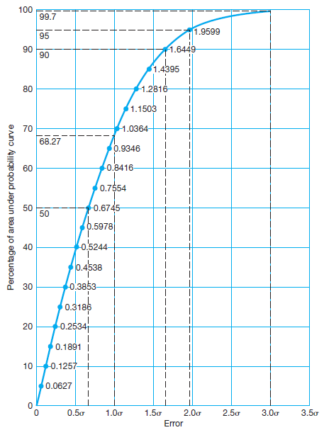
The probability of an error of any percentage likelihood can be determined using the following general equation:
\[E_{p}=C_{p}\sigma\]
where Ep is a certain percentage error and Cp the corresponding numerical factor taken from Figure 10.
The 50 percent error, or is the so-called probable error. It establishes limits within which the observations should fall 50% of the time. In other words, an observation has the same chance of coming within these limits as it has of
falling outside of them. The 90 and 95 percent errors are commonly used to specify precisions required on surveying (geomatics) projects. Of these, the 95 percent error, also frequently called the two-sigma error, is most often specified.